Highlighting AI Performance with a New Scale

When discussing how well an AI model performs on benchmarks, it’s common to talk about percentages or percentage points. However, these figures often obscure how significant the difference between two results really is, especially near the boundaries of 0% and 100%. In this post, I want to introduce an alternative: using a scale based on normal distribution, often referred to as a probit scale.

The Problem with Percentages and Percentage Points

Imagine comparing two models on a benchmark:

• Model A achieves 10 percent accuracy.
• Model B achieves 20 percent accuracy.

At first glance, this seems like a doubling of performance (“an increase from 10 to 20 percent”). However, percentage increases are difficult to generalize on the 0–1 (or 0–100%) scale, as it’s impossible, for instance, to double 60% to 120%.

Another way to describe this is an increase of 10 percentage points. While technically correct, this is not very informative. Moving from 0.10 to 0.20 is a much more significant improvement than from 0.45 to 0.55.

Probit: A Better Ruler for the Whole Scale

With a so-called probit transformation, we can translate results on the 0–1 scale to an infinite scale that accounts for the fact that differences near 0 and 1 matter more than those near the middle (e.g., 0.5).

From a technical perspective, the probit transformation is based on a normal distribution, and basically answers the question ”how far do I need to go on the normal distribution to cover X percent?”.

Let’s see how this works with the examples above:

• 10 percent (0.10) corresponds to a probit score of approximately –1.28 (which means that you’ll cover 10 percent of a normal distribution if you stop 1.28 standard deviations before the mid point).
• 20% (0.30) corresponds to a probit score of approximately -0.84 (meaning that you’ll cover 20 percent if you stop 0.84 standard deviations before the mid point).

The difference between the models is then 0.44 on the probit scale, illustrating the improvement in a more intuitive way.

Why Does This Matter?

The probit scale has two major advantages over percentages and percentage points:

1. Fairer Comparisons: A shift from 10% to 20% (0.77 probit points) is more significant than a shift from 50% to 60% (0.25 probit points).
2. Easier Cross-Benchmark Comparisons: The probit scale makes it easier to compare across different benchmarks. ”Model X improved records on benchmark A with 0.8 probit points, but only 0.15 probit points on benchmark B.”

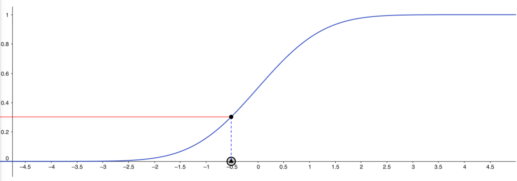
The graph below illustrates how percentages map to probit scores, showing how the scale stretches differences near the extremes while compressing those near the center.

Examples: o3 Benchmark Results

Here are some reported o3 benchmarks described as probit scores, along with previous benchmark records.

Result	Percetage (accuracy)	Probit Score
ARC record before o3	55%	0.13
o3 ARC result (high compute)	87.5%	1.15 (1.02 ahead)
o3 ARC result (not so high compute)	75.7%	0.70 (0.57 ahead)
o1 ARC result	21.2%	–0.80 (0.93 after)

Result	Percentage (accuracy)	Probit Score
FrontierMath record before o3	2%*	–2.05
o3	25%	–0.67 (1.38 ahead)

Result	Percentage (accuracy)	Probit Score
o1 on GPQA Diamond	78%	0.77
o3 on GPQA Diamond	88%	1.17 (0.40 ahead)

Conclusion

Using the probit scale to present AI results is a powerful tool that makes it easier to understand the true magnitude of differences between models. By transforming the results, we can avoid common pitfalls with percentages and percentage points and create a fairer, more intuitive metric.

What do you think about this way of presenting AI results? Share your thoughts in the comments below!

A technical note or two

• The probit scale (or actually the ”probit transformation”) is very similar to the logit transformation. Logit curves might be more familiar to some people working with ML. I suggest the probit scale here, because I think a normal distribution is easier to motivate (and understand), but a logit scale would work just as well.
• The idea of transforming values on a scale 0–1 to a scale plus/minus infinity using probit or logit isn’t new, and is for example used in educational test theory and psychology. Doing the same for AI benchmarks isn’t a revolutionary idea – it’s just applying something that works well in other fields in a new context.
• Note that this transformation is only relevant when measuring benchmark results on a scale 0–1 (or 0–100 percent). The Elo rating system used by LMSys, for example, can’t be transformed this way.
• *This kind of transformations are sensitive to noise in the very high/low ranges. The difference between 0.1 and 0.5 percent might seem negligible, but is 0.51 on the probit scale – roughly the same as the difference between 50 and 70 percent. This is a feature, not a bug, but means that noise in the very high/low regions will be amplified. (For example, the ”2%” result on the FrontierMath benchmark, in the table above, is pretty rough. It matters whether the actual value is 1.8% or 2.2%.)